
Abstract
As service lifetimes of electric vehicle (EV) and grid storage batteries continually improve, it has become increasingly important to understand how cells perform after extensive cycling. The multifaceted nature of degradation in Li-ion cells can lead to complex behavior that may be difficult for battery management systems or operators to model. Accurate characterization of heavily cycled cells is critical for developing accurate models, especially for cycle-intensive applications like second-life grid storage or vehicle-to-grid charging. In this study, we use operando synchrotron x-ray diffraction (SR-XRD) to characterize a commercially manufactured polycrystalline NMC622 pouch cell that was cycled for more than 2.5 years. Using spatially resolved synchrotron XRD, the complex kinetics and spatially heterogeneous behavior of such cells are mapped and characterized under both near-equilibrium and non-equilibrium conditions. The resulting data is complex and multifaceted, requiring a different approach to analysis and modelling than what has been used in the literature. To show how material selection can impact the extent of degradation, we compare the results from polycrystalline NMC622 cells to an extensively cycled single-crystal NMC532 cell with over 20,000 cycles—equivalent to a total EV traveled distance of approximately 8 million km (5 million miles) over six years.

This is an open access article distributed under the terms of the Creative Commons Attribution 4.0 License (CC BY, http://creativecommons.org/licenses/by/4.0/), which permits unrestricted reuse of the work in any medium, provided the original work is properly cited.
Accurate characterization and modelling of battery degradation has become a critical issue in the energy storage sector, as the adoption of electric vehicles (EVs) and grid-scale energy storage systems (ESSs) becomes increasingly widespread. Improved service lifetimes are making new applications possible, including vehicle-to-grid (V2G) storage and "second-life" repurposing of used EV battery packs in grid-storage facilities. While these applications have the potential to supply low-cost storage capacity to the grid, they require a comprehensive and accurate understanding of how degraded batteries behave after thousands of cycles and years of operation. The development of techniques that can characterize heavily degraded commercial cells operating under real-world conditions is critical to understanding the complex, multi-scale effects of battery degradation.
X-ray diffraction (XRD) has been widely used for decades to carry out in-situ and operando battery experiments. The first such experiments using an intercalation cell were done by Chianelli et al. in 1978, using a parallel-plate Li-TiS2 cell with an X-ray-transparent beryllium window. 1 This basic scheme, where the cell is designed for characterizing one electrode in reflection (BraggBrentano) geometry using a tube-based X-ray source, has since been employed for numerous operando battery experiments. The first cell designed for operando XRD experiments in transmission geometry was a single-layer pouch cell developed by Gustafsson et al. in 1992. 2 Many studies have since employed similar schemes, where in-situ cells are assembled in-house that are purpose-built for a given experiment. While these cells are optimized for collecting high-quality XRD data and are well-suited for short-term studies, they are not designed for cycling over the many weeks, months, or years required to study long-term degradation. Commercially manufactured cells, on the other hand, are ideally suited for studying long-term degradation, as they are reliable, highly reproducible, and represent real-world operating environments. Unfortunately, unmodified commercial cells are often not suitable for in-situ XRD experiments using lab-based diffractometers. 3 Advanced radiation sources are often required to for such experiments, especially for high-rate operando studies that require short measurement times.
In 2004, Rodriguez et al. used in-situ neutron diffraction to characterize lattice changes in a fresh, unmodified, commercial LiCoO2 (LCO) prismatic cell. 4 The first studies (to our knowledge) that used neutron diffraction to study long-term degradation in commercial cells were done by Helmut Ehrenberg's group in 2012, where operando experiments were used to show subtle changes in LCO lattice parameters for cycled LCO/graphite 18650 cells. 5,6
The first use of spatially resolved neutron diffraction to characterize a degraded commercial cell was done by Cai et al. in 2013. 7 In this study, The authors showed that the state of charge (SoC) of cycled LiMn2O4 (LMO) across the width of the cell was not uniform, with lower local SoC towards the edges of the cell. The authors also observed the splitting of the LMO (222) peak into two components during operando experiments: an "active" component that shifted during charge/discharge and a "non-active" component that shifted more slowly. This non-active component has since become a focus of similar studies on degraded cathodes.
More recently, high-energy synchrotron XRD (SR-XRD) has been adopted for operando battery experiments, though relatively few published SR-XRD studies exist that have used commercially manufactured cells to study degradation. Yu et al., used SR-XRD to map a large-format prismatic cell with a LiNixMnyCozO2 (NMC) cathode. 8 As with the study by Cai et al., Reduced local SoC at edges of the cell was observed after charge, and single-point operando measurements showed changes in current collector lattice spacing and strain during cycling. More recently, Leach et al. used a single-layer pouch cell (not commercially manufactured) to study the degradation of nickel-rich LiNi0.8Mn0.1Co0.1O2 (NMC811) after as many as 900 cycles at different C-rates. 9 These mapping experiments showed non-uniform distributions of active and non-active cathode after extended cycling (similar the results obtained by Cai et al. for LMO). However, the authors noted that the pristine cells also showed non-uniform SoCs just after formation, which was attributed to in-plane misalignment of the electrodes during cell assembly. These issues underscore the risks of using lab-built cells for such experiments.
Despite these challenges, most operando XRD studies of cathode degradation have used single-layer pouch cells or coin cells. In 2017, Liu et al. investigated fatigued NCA using specialized in-situ single-layer cells with PTFE seals that were designed for long-term cycling. 10 A kinetically hindered trailing "shoulder" was observed for the NCA (113) peak, similar to the behavior of LMO observed by Cai et al. Schweidler et al. showed a similar behavior in cycled LiNi0.85Mn0.15Co0.05O2/graphite single-layer pouch cells, where the fraction of the fatigued cathode increased over 750 cycles at full depth of discharge (DoD). 11 Scanning electron microscopy (SEM) images showed increased microcracking with cycling, while transmission electron microscopy (TEM) data showed the presence of disordered rock-salt layers that grew thicker during long-term cycling. The authors argued that for this Ni-rich material, the observed kinetically hindered component was likely due to a combination of cathode surface reconstruction that was accelerated by microcracking.
More recently, Xu et al. used NMC811/graphite coin cells with laser-thinned X-ray "windows" to carry out long-term cycling experiments. 12 After ∼350 cycles, a non-active NMC component was observed at low SoC that remained after charging. The authors used a three-component model to account for the different stages of degraded NMC, which they referred to as "fatigued," "intermediate," and "active." These three components were modelled as three phases in a Rietveld refinement, each of which was assigned a fixed lithiation state. The implicit assumption with this approach is that each of the three components has their own characteristic SoC that is reached after charge.
Among these examples, different profiles of non-active and/or kinetically hindered cathode components are observed for a variety of materials and cycling conditions. However, these studies all rely on simplified, single-layer cells to facilitate data collection and analysis. While these studies have provided valuable information on the kinetics of cycled cathodes, it's unclear to what extent the resulting conclusions and modelling assumptions can be applied to commercial cells. While there are studies that have employed commercial cells, they have focused mostly on static, full-cell mapping of SoC after charge/discharge. While this approach has also been informative, more involved operando experiments that explore changes in kinetic behavior and how they vary at different spatial scales have not, to our knowledge, been published in the literature. It should also be noted that cycle counts in most of these studies are in the hundreds of cycles, which is much shorter than the expected lifetimes of EVs and ESS facilities where cycle counts number in the thousands. As we will show, the situation can become significantly more complex in such degraded cells.
As part of previous studies, 13–15 our lab has carried out long-term cycling of commercially manufactured pouch cells containing polycrystalline NMC622 and natural graphite. These wound prismatic-shaped cells have been cycled extensively (thousands of cycles over more than two years) and have been thoroughly characterized using a combination of non-destructive electrochemical and imaging methods. Aggressively cycled cells from this matrix show complex and advanced degradation, including extensive cathode microcracking, electrode swelling, localized electrode delamination, and reduced amounts of excess electrolyte.
In the present study, we use spatially resolved, operando SR-XRD to characterize these cells at both near-equilibrium and non-equilibrium conditions. Using three cells from the matrix described above, we carry out a set of in-situ and operando mapping experiments to capture the complex, spatially heterogeneous changes occurring throughout the cell at different spatial scales. These experiments allow for both static and time-resolved mapping of fatigued cathode at near-equilibrium conditions, non-equilibrium conditions, and during open-circuit relaxation. This approach provides new insights into the behavior of heavily degraded cathode material under a variety of conditions. New approaches to quantifying and modelling are also presented, as the complexity and variability of this data requires a more empirical approach to modelling.
Previous studies have focused on characterizing polycrystalline cathode materials after cycling, but none included an investigation of strategies to mitigate microcracking — such as coatings, single-crystal cathodes, or other interventions used in industry. In this study, we compare the results from the polycrystalline NMC622 cells described above with results from a single-crystal NMC532 cell that has undergone over 20,000 cycles over a period of six years. Taken together, these experiments show just how complex and varied effects of degradation can be, and how they can be dramatically suppressed through the use of single-crystal cathodes.
Experimental Methods
Pouch cell preparation for polycrystalline NMC622 cells
402035-size wound prismatic-shaped pouch cells were manufactured by Li-Fun Technology (Zhuzhou, Hunan, China). Cells were shipped to our lab with no electrolyte, where filling, wetting, and formation were carried out. The cells consisted of an alumina-coated polycrystalline NMC622 positive electrode and a natural graphite negative electrode. Cathode composition was 96:2:2 (NMC622: PVDF binder: carbon black) with a single-layer active material loading of 19.3 mg cm−2 and double-layer thickness of 134 μm. The separator was made of polyethylene (PE) and coated with alumina on the cathode side. Anode composition was 95.4:1.3:1.1:2.2 (natural graphite: carboxymethyl cellulose binder: styrene butadiene binder: carbon black) with a single-layer active material loading of 13.6 mg cm−2 and double-layer thickness of 194 μm. The cell capacities at 4.3 V were ∼250 mAh during formation. After formation, the capacity at 4.1 V and C/10 was ∼220 mAh, which is the nominal capacity used for all C-rate calculations. The N/P ratio for most of these cells was balanced to the theoretical capacity at 4.5 V. One of the control cells (noted below) was made from identical materials, but came from a different batch (manufactured at the same time) that was instead balanced to 4.3 V. The polycrystalline cathode used in this work was composed of conventional secondary spherical agglomerations of smaller primary particles that are hundreds of nm in size.
Before cells were filled with electrolyte, they were cut open in an argon-atmosphere environment and dried under vacuum at 80 °C for 14 h. The cells were filled with electrolyte in an argon-atmosphere environment, then vacuum-sealed at a gauge pressure of −90 kPa and a temperature of 165 °C using a compact vacuum sealer (MSK-115A, MTI Corp.). The electrolyte used was 1.2 M LiPF6 in a 3:7 mixture by weight of ethylene carbonate (EC, BASF, 99.95%, <20 ppm water) and ethyl methyl carbonate (EMC, BASF, 99.9%, <20 ppm water), respectively. A VC211 ternary electrolyte additive blend was used, which consists of 2 wt% VC (BASF, 99.5%, <100 ppm water), 1 wt% TTSPi (Tokyo Chemical Industry Co., Ltd, >95.0%) and 1 wt% MMDS (Guangzhou Tinci Co. Ltd, 98.70%). After filling, the pouch cells were held at a constant voltage of 1.5 V for ∼24 h to ensure adequate wetting of the electrodes. Subsequently, the cells were charged from 1.5 V to 4.1 V at ∼C/20 and discharged to 3.8 V at 40 °C in a single formation cycle. The gas volume generated during formation was measured ex situ for all cells. Lastly, the cells were brought into an Ar-filled glovebox, cut open to remove any gases generated during formation, and re-sealed under vacuum.
Pouch cell preparation for single crystal NMC532 cells
Single-crystal NMC532 (grade BDA5000 from Zhenhua (China)) and artificial graphite (grade AML400 from Kaijin, China) were used in these cells. Cathode composition was 96:2:2:2 (NMC532: PVDF binder: carbon black: KS-6 conductive additive) with a single-layer active material loading of 21.1 mg cm−2 and double-layer thickness of 155 μm. The separator was made of PE and coated with alumina on the cathode side. Anode composition was 95.4:1.3:1.1:2.2 (artificial graphite: carboxymethyl cellulose binder: styrene butadiene binder: carbon black) with a single-layer active material loading of 12.2 mg cm−2 and double-layer thickness of 186 μm.
The cells were supplied dry, without electrolyte from Li-Fun and were filled and formed the same way as the polycrystalline NMC622 cells described above. Instead of the VC211 additive mixture used above, the electrolyte used in the NMC532 cells contained a mixture of 2% VC + 1% DTD (ethylene sulfate).
Long term cycling for NMC622 cells
NMC622 Cells were cycled continuously at 40 °C to an upper cutoff voltage (UCV) of 4.1 V. One cell was cycled continuously for approximately 2.5 years (2380 cycles) at a rate of C/5 to 100% DoD, using a voltage range of 3.0 V to 4.1 V. A second cell was cycled continuously for approximately 1.25 years to 25% DoD (3797 cycles) using a voltage range of 3.77 V to 4.1 V. A control cell from the same lot (formation-cycle only) was also included. Both cycled cells had checkup cycles approximately every 500 h. The checkup cycles consisted of full-range cycles (3.0 − 4.1 V) at C/10. Each cycle consisted of a CC-CV charge and a CC discharge. A CC-CV charge consists of a constant current (CC) charge from the lower cutoff voltage (LCV) to the UCV followed by a constant voltage (CV) hold at the UCV until the current decreased to C/20. A CC discharge consists of a constant current (CC) discharge from UCV to LCV.
Long term cycling for NMC532 cells
NMC532 cells were cycled between 3.0 and 4.2 V at 20 °C. Cells were cycled with a 1C CC charge with a C/20 CV hold, followed by a 1C CC discharge. C/20 checkup cycles were included every 100 cycles. Cells were cycled continuously for over 6 years, accumulating over 20,000 cycles.
Synchrotron X-ray diffraction (XRD)
All XRD data was collected on the Brockhouse X-ray Diffraction Sector (BXDS) on the Wiggler High-Energy (WHE) branch at the Canadian Light Source. 16 All experiments were carried out in transmission geometry, using a 2D flat-panel detector to capture Debye–Scherrer ring images. All data was collected using a beam energy of 55 keV and beam dimensions of approximately 200 × 50 μm (H x V). Static (non-operando) scans were collected using a large-area Perkin-Elmer detector with a sample-detector distance of 144 cm, while operando data was collected using a Dectris Eiger2 detector with a sample-detector distance of 120 cm.
Instrumental parameters were calibrated using a Lanthanum Hexaboride (LaB6−660a) standard reference material. Debye–Scherrer ring images were radially integrated using the GSAS-II software package. 17 Data management and plotting were carried out using custom Python code. Peak fitting was carried out using the FitYK software package. 18
Synchrotron computed tomography (CT) scans
CT scans were collected at the Canadian Light Source synchrotron facility using the Biomedical Imaging and Therapy Insertion Device (BMIT-ID) 19 and bending magnet (BMIT-BM) 20 beamlines. These beamlines provide a coherent, highly collimated X-ray beam with parallel geometry, allowing for enhanced contrast through propagation-based phase-contrast imaging. Imaging parameters are described in detail by Bond et al. 15 All scans were reconstructed using filtered back-projection and TIE phase retrieval, both implemented in the UFO-KIT software package. 21 All image analysis and visualization was carried out using the Avizo (Thermo Fisher) and Dragonfly (Object Research Systems) software packages. Thickness measurements were carried out manually, using five different points per measurement to calculate average values and errors (using a 95% confidence limit).
Results and Discussion
Three rectangular prismatic wound pouch cells with polycrystalline NMC622 cathodes and natural graphite anodes are characterized in this study:
- A "heavily cycled" cell (cycled continuously for 2.5 years at C/5 to 100% DoD),
- A "lightly cycled" cell (cycled continuously for 1 year at C/5 to 50% DoD)
- A control cell (formation cycle only)
Figure 1 shows the capacity fade and voltage polarization (ΔV) for the heavily cycled and lightly cycled cells. ΔV is the difference between the mean charge voltage and discharge voltage for a given cycle and is a measure of internal cell resistance. Sparse data points in these plots are from "check-up" cycles, where single cycles at C/10 to 100% DoD were carried out approximately once every 500 h. The capacity of the heavily cycled cell fades steadily to 76% of its original capacity after 2.5 years of cycling at 100% DoD, while the rate of capacity fade is much lower for the lightly cycled cell, retaining 96% of its original capacity after one year of continuous cycling at 25% DoD. The rate of increase in voltage polarization is also somewhat lower for the lightly cycled cell.

Figure 1. (a) Absolute and (b) normalized discharge capacity and ΔV vs time for two NMC622/NG pouch cells that are characterized in this study. Both cells were cycled at a rate of C/5 at 40 C to a UCV of 4.1 V. One cell was discharged to 25% DoD and cycled for 3800 cycles, while the other was cycled to 100% DoD and cycled for 2380 cycles. Sparse data points from each of the datasets are the data from 100% DoD, C/10 checkup cycles.
Download figure:
Standard image High-resolution imageBoth these cells (and the control cell) have been imaged extensively in previous work using nondestructive, in situ synchrotron CT. 14,15 Figure 2 provides a summary of CT data from these studies, showing the effects of mechanical cathode degradation at the cell level (top panel), and particle level (bottom panel). These images are 2D sections extracted from the 3D CT datasets, which can be thought of as digital "thin sections" with a thickness of one pixel. The grayscale values of these images correspond to the X-ray attenuation coefficients of the materials, where brighter pixels denote higher X-ray attenuation and darker pixels denote lower X-ray attenuation. At the particle level, extensive cathode microcracking in the heavily cycled cell (Fig. 2f) has caused massive swelling of cathode particles due to the reduced density of the fractured material. The geometry of the pore network is significantly altered, as micron-scale pore chambers are filled in by fractured, nano-porous cathode material. The darker overall grayscale values in Fig. 2f are also consistent with nanoscale microcracking that leads to lower density in the heavily cycled cell compared to the control cell. By contrast, the cathode from the lightly cycled cell (Fig. 2e) shows only subtle changes compared to the control cell (Fig. 2d), though there is a slight increase in thickness for the lightly cycled cell, and there appears to be a slightly higher number of visible cracks.

Figure 2. SR-CT data showing the effects of mechanical degradation at the cell level (a)–(c) and cathode particle level (d)–(f) for each of the three cells discussed in this study. The regions containing excess liquid electrolyte (and a gas pocket) are indicated in (a). More extensive CT data and analysis is provided in a separate publication. 15 Arrows in (d) and (e) indicate visible cracks in the cathode material.
Download figure:
Standard image High-resolution imageAll three cells were initially filled with excess amounts of electrolyte, as shown in the low-magnification CT scan of the control cell (Fig. 2a). After cycling, the amount of excess electrolyte is significantly reduced in the lightly cycled cell (Fig. 2b), while there is no sign of excess electrolyte at all for the heavily cycled cell. This depletion of excess electrolyte is consistent with the observed microcracking, as the increased total pore volume in the cathode would be expected to draw excess electrolyte into the jelly roll via capillary action. If the total pore volume of the electrode stack were to exceed the volume of electrolyte in the cell, localized dryout would begin to occur that could then spread and lead to rollover failure.
Other consequences of microcracking include loss of active electrode material (due to cracked particles becoming electrically disconnected) and an increase in the rate of surface-mediated parasitic reactions (due to the increase in exposed electrode surface area to electrolyte). One such reaction is the formation of disordered rock-salt phases with poor ionic diffusivity at the cathode surface. Taken together, these changes in particle size, pore network geometry, electrolyte distribution, electrical contact, and surface chemistry may all affect the kinetics of lithiation in potentially complex and varied ways.
To characterize the spatial variation of lithiation kinetics across the cell, SR-XRD mapping experiments were carried out under a variety of conditions. Practical considerations for conducting such experiments with commercial cells are first discussed. We then present static maps that show the near-equilibrium distributions of lithiation states and how they vary across the cell. From this data, we propose a simple method for estimating the fraction of inactive cathode material present at each point in space.
We then move to operando experiments that show how varied and complex the kinetic behavior of extensively cycled cells can be during operation. We propose a three-component peak fitting protocol to model the changing distribution of lithiation states over time and space. This approach provides a way to quantify the relative fractions of inactive, kinetically hindered, and fully active cathode material. The kinetic behavior of the cells during relaxation to open-circuit voltage (OCV) is then investigated at different spatial scales, and strategies for reducing and visualizing this data are proposed. Finally, operando SR-XRD is combined with high-resolution in-situ CT imaging to determine the extent to which microcracking—and the associated kinetic effects—can be supressed using a single-crystal cathode material.
Practical considerations for SR-XRD measurements of commercial cells
All SR-XRD experiments were carried out in transmission geometry using 2D flat-panel detectors to capture the Debye–Scherrer ring images. The small beam width (approximately 200 μm) allows for high-resolution spatial mapping of the cell, and the short acquisiton time (as little as 1 s per pattern in this study) allows for high-rate operando measurements. Figure 3 shows photographs of two experimental setups used for these experiments. Figure 3a shows the static experiment setup, where a large-area detector captures the full 360-degree arc of the Debye-Scherrer rings. For time-resolved experiments, a high-speed photon counting detector with a smaller physical area was used, which covered only one quadrant of the Debye–Scherrer rings. Details on these setups are provided in the experimental section and in the associated references.
In both cases, the cell was mounted on a 3D-printed holder using a 4-wire connection, as shown in Fig. 3c. The cell and holder were affixed to a high-precision translation stage that moves the cell in the plane perpendicular to the beam. Note that in both cases, a large sample-detector distance was used (144 cm for static measurements and 120 cm for time-resolved measurements). This was done to minimize peak broadening that arises when the sample thickness is large relative to the sample-detector distance. The cells used in this study are approximately 3.5–4 mm thick, which would yield significant peak broadening at smaller sample-detector distances. Initial testing was carried out using a lower beam energy of 35 keV and sample-detector distance of 47 cm. Figure 3d shows a comparison of peak broadening of the NMC (113) peak for the control cell (formation cycle only) at sample-detector distances of 47 cm and 144 cm (where 2θ values are converted to d-spacings for comparison). The beam energy was also adjusted to maintain the desired 2θ range, using an energy of 35 keV at the short distance (47 cm) and 55 keV at the large distance (144 cm).
For reference, a single layer of NMC622 was extracted from a dry pouch cell and measured at a sample-detector distance of 144 cm, representing a measurement with negligible peak broadening due to sample thickness. Compared to the single-layer peak (green), there is slight broadening due to cell thickness at a sample-detector distance of 144 cm, and significant broadening at 57 cm. Reducing peak broadening for these measurements is important, as many of the effects studied here involve closely spaced peaks.
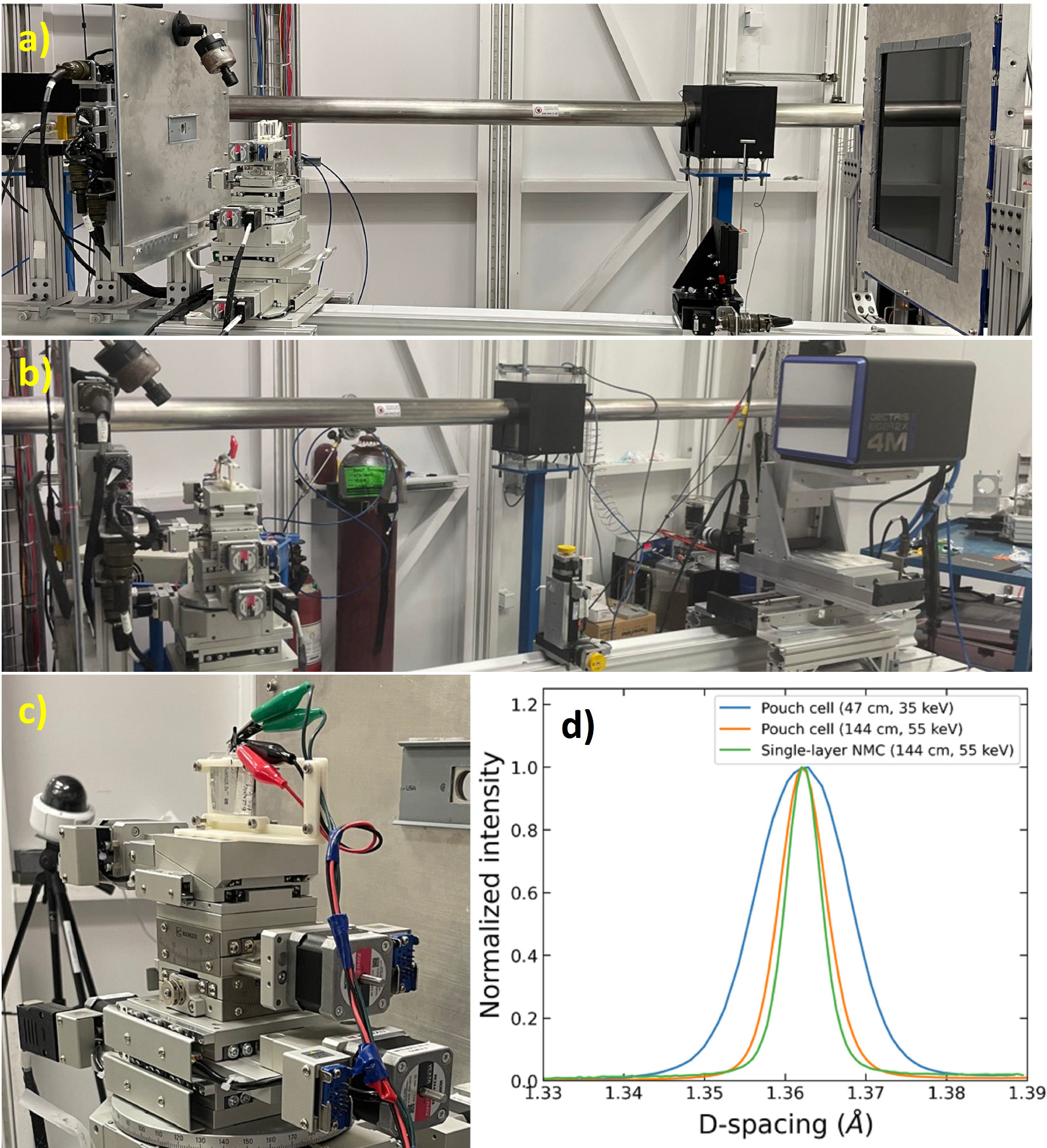
Figure 3. (a) XRD setup for in-situ pouch cell experiments using a large-area, low-speed detector. (b) XRD setup for operando measurements using a smaller-area, high-speed detector. (c) Closeup of pouch cell fixture. (d) Peak broadening of NMC (113) reflection due to cell thickness at different sample-detector distances and beam energies (compared to the peak width of a single layer of cathode material).
Download figure:
Standard image High-resolution imageFigure 4 shows an example of a full XRD pattern acquired from the control cell, using the static setup pictured in Fig. 3a. Since the beam passes through the entire electrode stack, reflections from all electrodes and current collectors are visible, with several overlapping peaks in the range of 5 to 8°. This study focuses mainly on the NMC (113) peak, as it is free from interference with these other peaks and its position has a near-linear relationship with cathode lithiation state. The lithiated graphite (00l) family of peaks (3 to 4°) is also analyzed in this study, as it is also free from interference and its relationship to lithiated graphite staging has been well characterized in the literature.

Figure 4. Overview of pouch cell XRD pattern collected at 55 keV. Peaks are assigned to electrode and current collector materials as labelled. The graphite (002) and NMC (113) peaks are the focus of this study.
Download figure:
Standard image High-resolution imageIn-situ SR-XRD mapping of cells under near-equilibrium conditions
To characterize the cells under near-equilibrium conditions, they were CC-CV discharged at C/5 to a minimum current of C/50 the day before data collection. Spatial line scans were then acquired with the cell at OCV, where XRD patterns were collected at regular increments across the width of the cell using a step size of 0.5 mm. This was repeated after CC-CV charge (at the same C-rates as above) to 4.2 V. This charge was carried out on the beamline without moving the cell to ensure the same points were probed at low and high SoC. Data was collected immediately after the CC-CV charge was completed. Figure 5 shows the resulting spatial line scan series of the control cell for the graphite (00l) and NMC (113) peaks at 3.0 and 4.2 V. The plots are colorized to highlight subtle changes in peak intensity. The y-axis of these plots shows the distance of each probe point from one edge of the cell, and each pattern is offset so that the background-subtracted baseline of that pattern intersects the y-axis at its corresponding position. Gray dashed lines for the lithiated graphite data (Figs. 5a and 5c) denote the positions of peaks that correspond to different stages of lithiated graphite, including stage 4 (least lithiated), stage 2 L, and stage 1 (most lithiated). For Figs. 5b and 5d, dashed gray lines denote the peak positions at 3.0 V and 4.2 V (respectively) for the NMC (113) peak. The 2θ values of these dashed lines—defined by the peak positions of the control cell at top and bottom of charge—are used as a reference for the cycled cells, which would be expected to have a narrower charging window after cycling under the same conditions.

Figure 5. Spatial distribution of XRD patterns for the control cell (formation cycle only). Plots show the distribution of lithiated graphite (00l) peaks (a), (c) and NMC (113) peaks (b), (d) collected after CC-CV discharge (a), (b) and charge (c), (d) to the indicated cutoff voltages. The positions of XRD probe volumes for each pattern are shown in green using a CT scan (e), (f). Dashed lines indicate positions of lithiated graphite staging peaks (a), (c) as well as those of NMC (113) peaks at 0% and 100% SoC. (g) shows a photograph of a dry cell that was disassembled and unwound to show a "taped-off" section of cathode at the core. Orange arrows highlight this region in the photo, which corresponds to the area highlighted by the dashed orange ovals in the CT scan (e), and corresponding NMC (113) data (d). (h) shows a magnified region from the CT scan of the jelly roll core, with red arrows highlighting the inner layer of the anode that has no adjacent cathode. As with the inactive cathode, the corresponding area on the full-cell CT scan (e), and lithiated graphite (00l) data are highlighted with a dashed red circle.
Download figure:
Standard image High-resolution imageFrom a CT scan of the control cell, a 2D cross section (Fig. 5e) and longitudinal section (Fig. 5f) were extracted. There is a gradual, "wavy" variation in the grayscale intensity in Fig. 5f, which is due to the copper foil at the center of the cell that weaves in and out of the extracted 2D plane. In both 2D sections, green lines and dots are overlayed, which show the probe point locations at which the XRD patterns were acquired, with each line/dot corresponding to its respective pattern in Figs. 5a–5d. The bottom edge of the cell in these images is defined (arbitrarily) as the edge from which all distances across the width of the cell are measured. The locations of these XRD probe positions within the CT scan were determined by acquiring absorption maps on the XRD beamline and raster scanning the beam across the cell at high spatial resolution (0.2 mm step size) while measuring the transmitted X-ray beam intensity using a photodiode on the beam stop. These absorption maps were then aligned digitally with the CT scans so that any XRD data collected at a known set of sample-stage motor coordinates could then be located in the CT scan. This mapping and alignment procedure was repeated for all cells.
For the control cell, the NMC (113) data is spatially uniform, both in terms of peak position and shape. In Fig. 5d however, there is a small region at 12 to 14 mm from the edge (highlighted with a dashed orange circle) where a small portion of cathode appears to be at a lower SoC (more lithiated) than the rest of the cell. Figure 5g shows a photo of a disassembled dry pouch cell (from the same batch of cells) that was unwound to show the innermost layer of cathode at the core. A piece of green tape holds the cathode layer in place, which overlaps with the edge of the cathode, covering a 2 mm section and sealing it off from the anode. This innermost cathode layer is highlighted in the CT scan (Fig. 5e) and corresponds to the same region where the lower-SoC cathode was detected in the XRD data. The low SoC (high lithiation state) of the anomalous cathode material in this region is consistent with pristine cathode material that would have been "taped off" during cell winding and unable to delithiate during cycling (except perhaps by slow lateral diffusion). This result shows that these types of transmission XRD measurements are sensitive to differences occurring in even a single layer of electrode material buried within the cell.
The lithiated graphite (00l) peak positions and areas are uniform across the width of the cell. At 3.0 V, the graphite is almost all stage-4, which then transitions to a mix of stage-2/2L and (to a lesser extent) stage-1 graphite at 4.2 V. Note that these cells were balanced to 4.5 volts, which is why so little stage-1 graphite is present after charging to 4.2 V. A small set of anomalous peaks is also visible in the range of 12.5 to 17.5 mm from the cell edge (both at 3.0 and 4.2 V). This region corresponds to the innermost turn of the cell, where a high-resolution CT scan (Fig. 5h) shows that graphite is present in the inner core without any adjacent cathode (as indicated by red arrows). The corresponding regions in the full-cell CT scan (Fig. 5e) and lithiated graphite (00l) data (Fig. 5a) are highlighted with dashed red ovals. As with the cathode, this shows that a single layer of graphite at a different state of lithiation can be detected under these conditions, despite the lower scattering factor of carbon.
The spatial uniformity shown in this cell is not a given, especially when cells are made by hand or using lab-scale equipment. Problems with electrode alignment, stack pressure distribution, electrolyte wetting, etc can all give rise to non-uniform behavior that can produce inaccurate or even misleading results. This was noted by Leach et al., who showed that even a small (∼300 μm) electrode misalignment in their hand-made pouch cell could generate significant variance in cathode lattice parameters. 9 The reliability and reproducibility of commercially manufactured cells is especially important for experiments at major facilities, such as synchrotrons or neutron sources, where time is often limited and cell malfunction or failure need to be avoided.
Figure 6 shows spatially resolved data for the lightly cycled cell (25% DoD at C/5 for 1.25 years) using the same general scheme as Fig. 5, where the probe positions of graphite (00l) and NMC (113) peaks are mapped to a CT scan of the cell. The XRD data is similar to the control cell, though the NMC (113) peaks are slightly offset from the dashed gray lines that indicate the peak positions at 3.0 V and 4.2 V for the control cell. This is likely due to the capacity loss in the cycled cell, which would lead to a narrower window of lithiation state over the same voltage range.

Figure 6. Spatial distribution XRD patterns for the cell cycled to 25% DoD for 1.25 years (3800 25% DOD cycles). Plots show the distribution of graphite (00l) peaks (a), (c) and NMC (113) peaks (b), (d) collected after CC-CV discharge (a), (b) and charge (c), (d) to the indicated cutoff voltages. The positions of XRD probe volumes for each pattern are shown in green using a CT scan (e), (f). Dashed lines indicate positions of graphite staging peaks (a), (c) as well as those of NMC (113) peaks at 0% and 100% SoC from the control cell data in Fig. 5.
Download figure:
Standard image High-resolution imageInactive graphite is visible at the top end of the line scan and there also appears to be inactive cathode material in the region 10 to 15 mm from the edge of the cell. Unlike the control cell, these inactive peaks are visible in both the 3.0 V and 4.2 V data and can be seen over a larger area than the 2 mm section that is "taped off" in these cells. Given that this cell was cycled only between 75% and 100% SoC, some of the cathode in this taped-off region may have slowly become delithiated via lateral diffusion into the surrounding material, which would have been at a lower average state of lithiation during cycling. A small region around 3 to 4 mm from the edge in Fig. 6b also appears to contain inactive cathode. A quantitative comparison of peak areas in these regions (see Fig. 9 below) shows that there is indeed more inactive material in this cell than the control cell, however, it is remarkable how similar the two cells are after one of them was cycled for 1.25 years (3800 25% DOD cycles) at high average SoC.
Figure 7 shows spatially resolved XRD data for the heavily cycled cell (100% DoD at C/5 for 2.5 years, 2370 cycles). In contrast to the control and lightly cycled cells, the distributions are clearly multimodal, with widely varying peak shapes and positions across the cell. Trailing peaks resembling the "sluggish" or "fatigued" cathode described by Kleiner et al., 22 Liu et al., 10 and Xu et al. 12 are visible throughout the NMC (113) spatial series at both 3.0 V and 4.2 V. Using operando experiments at higher C-rates (discussed below) we will show that trailing peaks with slow kinetics are indeed observed during charge/discharge at faster rates, but the peaks that are left behind after CC-CV discharge are stationary and likely represent disconnected cathode material. In this study, we will refer to these stationary peaks as "inactive" NMC.

Figure 7. Spatial distribution of XRD patterns for the cell cycled to 100% DoD for 2.5 years. Plots show the distribution of lithiated graphite (00l) peaks (a), (c) and NMC (113) peaks (b), (d) collected after CC-CV discharge (a), (b) and charge (c), (d) to the indicated cutoff voltages. The positions of XRD probe volumes for each pattern are shown in green using a CT scan (e), (f). Dashed lines indicate positions of lithiated graphite staging peaks (a), (c) as well as those of NMC (113) peaks at 0% and 100% SoC from the control cell data in Fig. 5.
Download figure:
Standard image High-resolution imageSome amount of inactive NMC appears at every point across the width of the cell, but it appears most concentrated near the center, in the region approximately 8 to 13 mm from the edge. In this same region, the lithiated graphite (00l) data at 3.0 V also shows a corresponding localization of graphite that has not been fully delithiated after discharge, with peaks visible in transitional phases between stage 2 L and stage 4. After charging to 4.2 V, the same region shows very little stage-1 lithiated graphite compared to other parts of the same cell, as does a smaller region at 3 to 5 mm from the cell edge. These regions of less-lithiated graphite appear to correlate spatially to higher concentrations of inactive NMC (113) peaks. This correlation can be explained by the localized loss of lithium that would be sequestered in inactive cathode particles, making it unavailable for lithiation of graphite at the same position in the cell. The extensive cathode microcracking shown in Fig. 2f suggests that the observed inactive cathode is likely due to electrically disconnected particles.
In addition to the concentration of inactive cathode around the center of the cell, there is also a slight concentration of inactive cathode in the region at 3 to 6 mm from the edge. This region corresponds to a damaged portion of the jelly roll, where delaminated cathode is visible in the CT scan. This cathode damage is caused by swelling of the jelly roll into the core of the cell, which becomes distorted as it wraps around the current collector tabs (described in detail by Bond et al.). 14,15
Assuming the inactive cathode peaks are in fact static, a simple procedure can be used to isolate and quantitatively estimate the inactive fraction of cathode using the NMC (113) data. Figure 8a shows an example of this procedure. Ideally, if the peaks at 3.0 V (blue) and 4.2 V (red) were completely separated from one another, the inactive fraction could be isolated by computing the intersectional area (colored yellow in Fig. 8a) of the two patterns. Despite efforts to reduce peak broadening and increase peak separation, some overlap remains between the 0% and 100% SoC peaks. The intersectional peak areas for all three cells are shown in Figs. 8b–8d. The intensity scale for these plots is the same as Figs. 5–7. In all three plots, a small, sharp peak is visible near the midpoint (near 9.55°), where the low-SoC and high-SoC active peaks intersect. Below this point, the isolated inactive fraction is defined by the low-angle 4.2 V data, and above the point, it is defined by the high-angle 3.0 V data.

Figure 8. (a) Illustration of peak areas used for estimation of positive mass loss, using the NMC (113) peaks acquired at bottom of charge (blue) and top of charge (red). The intersectional area of these two peaks is used to estimate the fraction of inactive material, which is shaded in yellow. Spatial distributions of these intersectional areas are shown for (a) the control cell (b) the cell cycled to 25% DoD for 1.25 years, and (c) the cell cycled to 100% DoD for 2.5 years. Dashed lines denote the positions of active peaks at 0% and 100% SoC from the control cell data in Fig. 5.
Download figure:
Standard image High-resolution imageThese plots allow us to more easily visualize the spatial distribution and peak positions of inactive cathode material. For the heavily cycled cell, the inactive peaks tend to be at a higher SoC (low lithiation state), as does much of the inactive cathode component in the lightly cycled cell. A possible explanation for this trend is that disconnection events may preferentially occur as the particles shrink to smaller volumes during delithiation.
In the control cell data—where there should be no inactive material except for the taped-off region noted above—there is a slight residual background visible at all points in Fig. 8b, due to the overlapping "tails" of the active peaks. This background is present in all three cells and contributes to an overestimate of the inactive cathode fraction. For the heavily cycled cell data, there is an asymmetric tail on the low-angle side of the isolated inactive cathode peak. While the overlapping tails of the active peaks mentioned above likely contribute some portion of this low-angle feature, it could also be caused by kinetically hindered material or disconnected cathode particles in a high lithiation state. 14 Restricted kinetics plays a much more significant role at higher C-rates, yielding much more noticeable low-angle shoulders in operando data, which is discussed in detail below. For now, we simply treat this feature as part of the inactive cathode.
The peak areas of the isolated inactive components shown in Figs. 8b–8d can be used to quantitatively estimate the inactive fraction of cathode material (also referred to as the positive mass loss fraction). Here, we calculate this fraction using Eq. 1, where Aintersect is the intersectional area of the high- and low-SoC peaks, A3.0V is the area of the low-SoC peak (excluding the intersectional area) and A4.2V is the area of the high-SoC peak (also excluding the intersectional area). These areas are illustrated in Fig. 8a. For the denominator of this fraction, the average of the low-SoC and high-SoC areas is used rather than simply one area or the other. These two peak areas are generally similar, but this averaging is done to reduce any bias that could result from a discrepancy between them.

For the control cell, in the regions where there should be no positive mass loss, this positive mass loss fraction is calculated to be 8.7% on average. As mentioned above, this results from overlapping tails of the low-SoC and high-SoC active peaks. To partially correct for this overestimation, this control cell value (8.7%) was subtracted from all positive mass loss fractions. For cycled cells, the overestimation due to active peak overlap is likely to be more significant, where peaks are broader, and the cell is thicker. Subtracting the control cell values from this data is likely insufficient to fully correct for the bias when peak broadening is significant, but it should reduce the degree of overestimation for cycled cells without overcorrecting.
Figure 9 shows the spatial distribution of positive mass loss fractions calculated for all three cells (and overlayed on their respective CT images). The average mass loss fractions were calculated to be 1.8% for the control cell, 2.8% for the lightly cycled cell, and 28.8% for the heavily cycled cell. The positive mass loss fraction for the two cycled cells was also calculated using dQ/dV fitting by Gauthier et al., yielding a mass loss fraction of 7.1% for the lightly cycled cell and 17.1% for the heavily cycled cell. 13 Note that the value calculated using dQ/dV fitting is higher than the value calculated here for the lightly cycled cell, but lower for the heavily cycled cell. The discrepancy between these two methods could be due to spatial sampling, since only one "slice" of the cell was analyzed using XRD, which also excluded the cell's outer edges. For the heavily cycled cell, there is significant spatial variability across the width of the cell, with mass loss fraction values ranging from 23% to 54%, which is much larger than the discrepancy between the values obtained using XRD and dQ/dV. However, given the errors and tendency to overestimate as discussed above, the approach outlined here should be regarded as semi-quantitative.
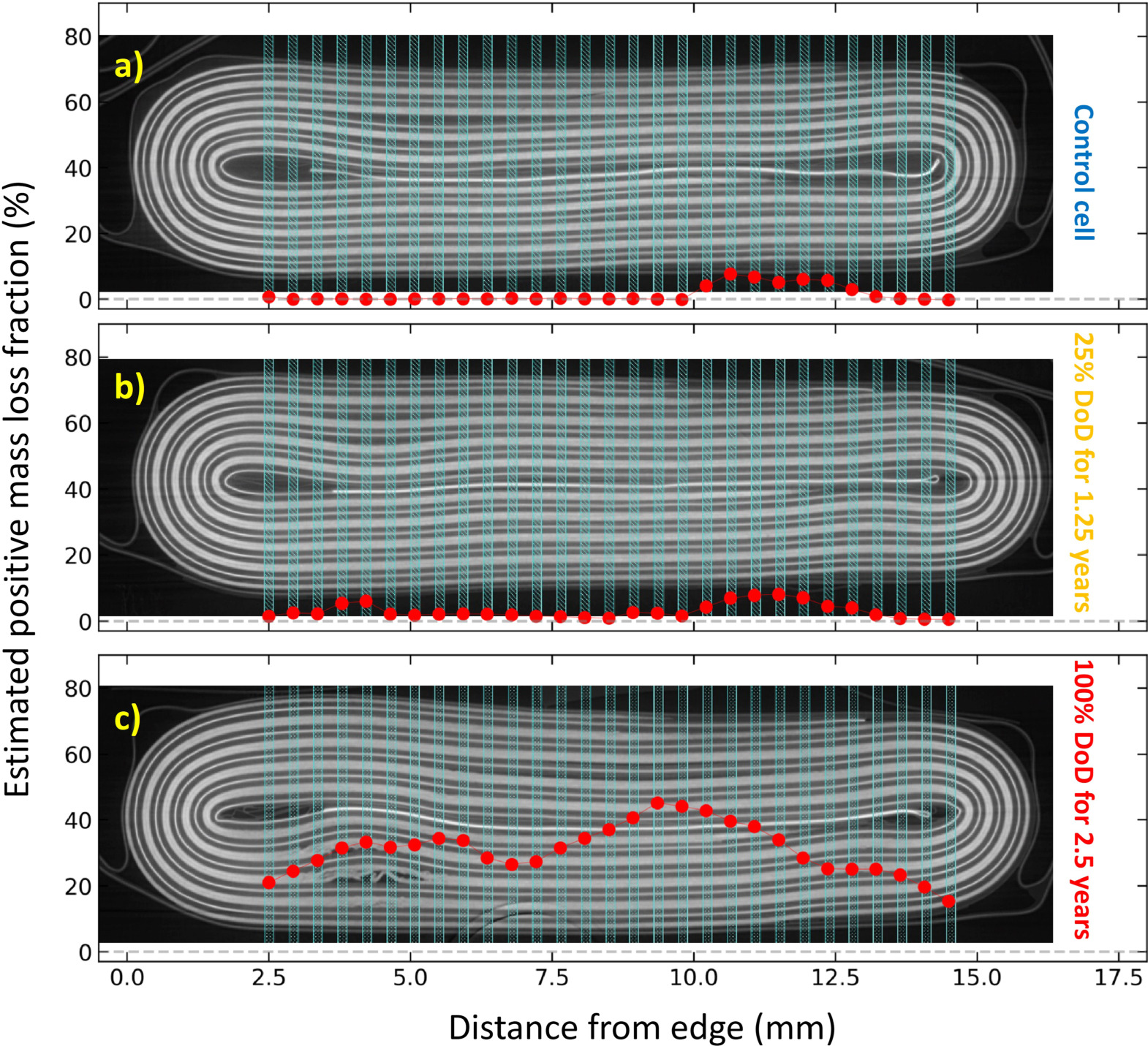
Figure 9. Plots of estimated mass loss for (a) the control cell (b) the cell cycled to 25% DoD for 1.25 years, and (c) the cell cycled to 100% DoD for 2.5 years. These values were obtained by integration of the intersectional peak areas shown in Fig. 8. The plots are overlaid on CT scans of the cells, showing which positive mass loss value corresponds to each XRD probe position in the cell.
Download figure:
Standard image High-resolution imageOperando SR-XRD mapping of cells during charge
To study the non-equilibrium behavior of the cycled cells, operando experiments were carried out where spatially resolved sets of XRD patterns were acquired repeatedly over time as the cell was charged to 4.2 V at a rate of C/5 (at room temperature). Prior to data acquisition, cells were CC-CV discharged to 3.0 V using a CC current of C/5 and a minimum CV current of C/20, then left at OCV overnight. Figure 10 shows the resulting time-resolved data for the NMC (113) peak collected for both the control cell (upper row) and heavily cycled cell (lower row). Each plot contains a time series collected at the indicated distance from the edge of the cell. The y-axis for these two plots has been adjusted so that the time scale is the same for both sets of data, which was shorter for the heavily cycled cell due to capacity fade and increased polarization.

Figure 10. Time-resolved plots showing the evolution of the NMC (113) peak during CC charge at C/5 from 3.0 V to 4.2 V, where the top row (a) shows data for the control cell and the bottom row (b) shows data for the cell cycled to 100% DoD for 2.5 years. Each individual plot shows data that was collected at the indicated distance from the edge of the cell. For the cycled cell, gray dashed lines indicate the position of peaks that appear to be static, indicating the presence of inactive cathode material.
Download figure:
Standard image High-resolution imageThe control cell shows uniform, spatially homogeneous behavior across the cell, with unimodal peaks moving at a constant rate from low to high 2θ. By contrast, the heavily cycled cell shows complex, heterogeneous behavior, with a multimodal distribution of peaks moving at different rates. The movement of these peaks is highly nonlinear in some cases. For example, at 11 mm from the cell edge, there appear to be two peaks that are initially stationary, but after approximately 2 h the low-SoC peak rapidly delithiates as if it was initially disconnected and suddenly became reconnected. At 7 mm from the edge, there appears to be one inactive peak and two active peaks that all delithiate at different rates. At 13 mm from the edge, there appear to be multiple stationary peaks and one or more active peaks. Given that these cells are so uniform in the control cell, the degree of variation across the cycled cell is truly remarkable. One thing that all the spatial points in the cycled cell appear to have in common is the presence of at least one stationary peak (highlighted in Fig. 10b with dashed gray lines). This further supports the assumption from the nearequilibrium data analysis that the peaks which are "left behind" after CC-CV charge/discharge are likely due to inactive cathode material.
As discussed in the introduction, previous studies have taken various approaches to modelling fatigued cathode material. Many of these relied on static models, such as the 3-component model used by Xu et al. and Leach et al., where the "active" component is assumed to be the most delithiated peak after charge, the "intermediate" component is the next most delithiated, and the "fatigued" component is the least delithiated. In these studies, each of the three components was assigned a fixed lithiation state, which was then used to carry out Rietveld refinement and quantify the relative fractions of each component after different amounts of cycling. This approach fit the experimental data well for NMC811/graphite coin cells that were cycled approximately 1000 times. However, these assumptions are not applicable to the heavily cycled cell studied here, as the presence of inactive cathode at spatially varying states of lithiation would yield misleading results. The complex, nonlinear kinetic behavior shown here also makes such an approach impractical.
In this study, we suggest a different approach for modelling this type of data. Rather than attempt full Rietveld refinement, single-peak fitting of the NMC (113) peak can be carried out using a few simplifying assumptions. This is demonstrated using the operando data from one of the spatial points in Fig. 10b (at 9 mm from the edge of the cell) as an example. The same model is then used to fit the near-equilibrium spatial mapping data of the heavily cycled cell showed in Fig. 7.
The first assumption for this approach is that an inactive peak is present, which will remain fixed throughout the time series data. As shown in Fig. 8d, most of the inactive NMC (113) peaks tend to be at higher 2θ, making them easier to extract from the initial-state (bottom-of-charge) data. Figure 11a shows the initial-state data at the beginning of charge (after CC-CV discharge to C/20), which can be modelled reasonably well using two pseudo-Voigt peaks. We assume that the higher-angle peak is inactive and will be fixed at all times. Figure 11b shows the end-state data after the C/5 charge to 4.2 V. Attempting to model this data with two peaks produces a poor fit, and there appears to be a significant low-angle component missing from the model. If we add a third peak, where the parameters for the inactive peak are fixed (from the initial fit of the 3.0 V data), and the parameters of the other two peaks are refined, a good fit can be achieved (as shown in Fig. 11d). Since this cell was only CC charged at C/5 with no CV top-up step, most of this low-angle peak is likely due to active material that is kinetically hindered. We label this peak as "semiactive," while the other two peaks are labelled "active" and "inactive," respectively. Note that if we had attempted to model the 4.2 V data assuming the highest-SoC peak to be the most active and lowest-SoC peak to be the most fatigued, we would have obtained misleading results. A three-component model can also be used to fit the data at 3.0 V, but adding a low-angle peak at that stage contributes little to the overall model.

Figure 11. Results of peak fitting for the NMC (113) peak for the cell cycled to 100% DoD for 2.5 years (using data collected at 9 mm from the cell edge). The top row (a), (b) shows results of fitting with a two-peak model and a fixed inactive peak, while the bottom row (c), (d) shows the fit for the same data using a three-component model. The left column (a), (c) shows data collected at 3.0 V and the right column (b), (d) shows data collected at 4.2 V.
Download figure:
Standard image High-resolution imageUsing the three-component model described above, every time point in the series was fit using the following procedure (an illustration of this procedure is provided in Fig. S20):
- 1.The initial time point was fit using three components.
- 2.The parameters of the inactive peak from the first time point were fixed and this static peak was copied to all other time points.
- 3.For the second time point, the active and semi-active peaks were fit using the parameters of the first time point as initial guess values that were then refined.
- 4.This process was repeated for each subsequent time point until the end of charge, where the fitted parameters from each point was used as the initial guess for the next point.
Figure 12 shows the results of this fitting, including a plot of separate components (Figs. 12a–12c, a combined plot with all components (Fig. 12d), and the resulting fit of the model at each point (Fig. 12e). In Fig. 12c, the active peak appears to spread out as the charge progresses, until just before the 2.0 h mark where it suddenly jumps to a higher angle and becomes narrow again. At the same point, the semi-active peak in Fig. 12b, goes from being negligibly small to a significant fraction of the model. Although the active and semi-active peaks are essentially combined into one peak at the start of charge (where they are both in a near-equilibrium state), the active peak begins to pull away from the semi-active peak as the cell is charged, and a single peak becomes insufficient to model both components.

Figure 12. Results of peak fitting the entire charge cycle for the cell cycled to 100% DoD for 2.5 years (using data collected at 9 mm from the cell edge). The top row shows the separate components of the model (a)–(c) and all components plotted together (d), as well as the resulting fit of the combined model to the time-resolved data (e). From these fitting results, the area fraction of each component (f) was calculated over the charge cycle, as well as the peak center positions (g). For both plots, boxes with blue dashed lines indicate the regions where the semi-active component does not contribute significantly to the model.
Download figure:
Standard image High-resolution imageFigure 12f shows the evolution of the peak area fractions for each of the model components over the course of the charge. The active peak area fraction is essentially constant until the 1.5 h mark, at which point it sharply decreases at the same point that the semi-active peak area fraction sharply increases. Both peak areas then converge back to the same value (∼25.5%). At every point in time, the combined peak area is essentially constant, with the sum of the two peak area fractions confined to a range of 54.7% to 56.8% throughout the charge. At this position in the cell, the largest of the three components is in fact the inactive fraction (43.3%), with the remaining cathode split evenly between the semi-active (25.3%) and active (25.5%) components. Figure 12g shows the peak center positions of all model components, both in terms of 2θ (left y-axis) and estimated SoC (right yaxis), which were calculated using the near-equilibrium charge endpoints of the control cell shown in Fig. 5. A dashed blue box outlines the region where the SoC of the semi-active component is less than 0%, indicating that it is not physically meaningful in this region. The same dashed blue box in Fig. 12f also shows that the contribution of the semi-active peak is close to zero over the same interval. Once the semi-active component becomes a relevant contributor to the model, its SoC changes very slowly as the cell is charged.
To model the static (near-equilibrium) data for the heavily cycled cell, the spatial line scans shown in Fig. 7 were fit using a similar approach to the one described above. NMC (113) peaks for each point in the 3.0 V line scan were first fit using a two-component model, then the parameters of the higher-angle peak were fixed and copied to the corresponding 4.2 V data. The 4.2 V data was then fit using a three-component model, assuming the higher-angle peak is the active component and the lower-angle peak is the semi-active component. Figure 13 shows the results of this modelling (using a similar scheme to Fig. 12). The "semi-active" fractions in Fig. 13b are much smaller compared to those in Fig. 12b, indicating that most of the kinetically hindered cathode that remained after CC charge at C/5 can be fully delithiated using a CC-CV charge. The peak area fractions in Fig. 13f show that the active fraction is much larger than the semi-active area fraction after CC-CV charge, while the two fractions were essentially equal after CC-only charge at C/5.

Figure 13. Results of peak fitting the spatially resolved data for the cell cycled to 100% DoD for 2.5 years. The top row shows the separate components of the model (a)–(c) and all components plotted together (d), as well as the resulting fit of the combined model (e). From these fitting results, the area fraction of each component (f) was calculated, as well as the peak center positions (g).
Download figure:
Standard image High-resolution imageThis peak fitting approach provides another way to calculate the positive mass loss fractions that were previously estimated using the peak intersection method outlined in Fig. 9. The values and spatial profile of the inactive area fractions calculated using peak fitting are very similar to those shown in Fig. 9c. The mean active mass fraction calculated using peak fitting was 29.9% (compared to 28.1% using the peak intersection method). Note that the spatial profile of the inactive peak area fractions is highly anticorrelated to the active area fractions.
From this data, the mean active peak area fraction was found to be 65.4% and the semi-active peak area fraction was only 4.63% after CC-CV charge. Compared to the active and semi-active peak area fractions after CC charge at C/5 (28.5% and 28.3%, respectively) it is clear that a significant portion of the kinetically hindered component that was incompletely delithiated after CC charge at C/5 has now been fully delithiated.
Figure 13g shows the spatial distribution of peak center positions of each component, which are fairly constant across the width of the cell. The average inactive peak center was 9.58°, equivalent to an SoC of 64.7%. This allows us to quantify the observation made previously that the inactive material exists at a high SoC, which would be consistent with electrical disconnection of shrinking cathode particles. The active component appears to be almost fully delithiated after CC-CV discharge, with a mean peak position of 9.62° (99.4% SoC), while the mean peak position of the semi-active component is 9.50° (4.22% SoC). The plots of both peak positions and peak area fractions for the semi-active component show several sharp, discontinuous drops across the cell. At these points, the peak area fraction drops to almost nothing at the same points where the peak position drops to below 0% SoC. This suggests that the semi-active component is not present at those points (or at least does not contribute significantly to the model). At these points, a two-component model would provide a reasonable approximation under near-equilibrium conditions.
High-speed operando experiments and OCV relaxation
In this section, we investigate the non-equilibrium behavior of the cells during OCV rest and use high-spatial-resolution operando mapping to better capture the scale of kinetic variations. Very few examples exist in the literature where XRD has been used to monitor local lithiation states during OCV relaxation. Liu et al. carried out an experiment using an NCA/Li-metal gasket-sealed coin cell that was cycled ∼90 times, then charged to 4.5 V and left at OCV for 10 h. 10 They acquired single-point XRD patterns before and after the OCV rest period, which showed that the single NCA (113) peak that had separated into two peaks during charge had then merged back into a single peak after OCV relaxation.
To characterize OCV relaxation in our cycled pouch cells, experiments were carried out using a similar time-resolved mapping approach as shown in Fig. 10 (where repeated line scans were acquired at regular intervals). The recent availability of a high-speed Eiger photon counting detector on the BXDS beamline allowed us to greatly increase both the time resolution and number of points measured during these experiments. This made high-rate cycling and 2D mapping possible, which were both exploited for these experiments.
To monitor relaxation during OCV rest, cells were CC charged from 3.0 V to 4.2 V at a rate of C/3 (at room temperature), followed by an OCV rest period that was terminated after the cell appeared to reach equilibrium. For the lightly cycled and heavily cycled cells, this was followed by a C/3 discharge and OCV rest. Prior to data collection, cells were CC-CV discharged to 3.0 V (to a minimum current of C/20), then left overnight. Figure 14 shows the charge curves of the three cells followed by a period of OCV rest. The control cell (Fig. 14a) charged for nearly 3 h and the voltage relaxed rapidly after the charging current was terminated. It should be noted that a different control cell was used for OCV relaxation experiments than that used for previous experiments. The new control cell contained the same materials (polycrystalline NMC622 and natural graphite) and was manufactured in the same run as the other cells in this study, but was balanced to 4.3 V instead of 4.5 V. The only notable difference in the data is that the extent of graphite lithiation in this cell is greater than that of the control cell used in the previous sections.

Figure 14. Voltage curves for (a) the control cell (b) the cell cycled to 25% DoD for 1.25 years, and (c) the cell cycled to 100% DoD for 2.5 years that were charged at a nominal rate of C/3 (73.3 mA), followed by an OCV rest. Dashed gray lines indicate the end of the charging stage.
Download figure:
Standard image High-resolution imageCompared to the control cell, the lightly cycled cell (Fig. 14b) shows a slightly more polarized charge curve and a more gradual relaxation during OCV rest. By contrast, the heavily cycled cell (Fig. 14c) shows a significantly polarized charge curve, reaching 4.2 V after just over an hour, followed by a very gradual relaxation to a much lower OCV than the other two cells. Even after ∼5 h of OCV rest shown in Fig. 14c, changes in the XRD patterns were still observed and the cell was monitored for a full 10 h before terminating the experiment.

Figure 15. Data collection patterns used for operando XRD experiments. The "low-resolution" line scan pattern (red) was used to cover a large region (10 mm with 2.0 mm spacing), while a high-resolution 2D grid (yellow) was used to map a smaller region (2.0 × 2.0 mm, with 0.2 mm spacing). A strip of points from the high-resolution grid is highlighted (light blue), which was used to characterize the space between low-resolution endpoints. The patterns are overlaid on a CT scan of the control (formation-only) cell. Points are numbered from left to right as indicated.
Download figure:
Standard image High-resolution imageDuring these experiments, two types of spatial mapping scans were carried out: a low-resolution line scan and a high-resolution 2D grid scan. Figure 15 shows a schematic of where on the cell these two scans were collected. The low-resolution line scan (shown in red) was collected with a step size of 2.0 mm—similar to the line scan shown in Fig. 10. The high-resolution 2D scan consists of a 10 × 10 grid with a step size of 0.2 mm. The C/5 time-resolved data in Fig. 10 showed significant differences between adjacent points that were just 2 mm apart. To investigate the region between these points, the 2D grid was positioned such that the endpoints of one of the rows (highlighted with a blue box in Fig. 15) coincided with two adjacent points in the low-res line scan.
For the heavily cycled cell, time-resolved experiments with low-resolution line scans were at first collected separately from the high-resolution 2D grid scans. For the control cell and lightly cycled cell, the sample stage motors were instead programmed to alternately collect low-resolution line scans and high-resolution grid scans during experiments. To complete both scans and return to the same point, a time interval of approximately 325 s (5.3 mins) was required. The time interval of the 2D grid scans for the heavily cycled cell was slightly shorter, at 260 s (4.3 mins). The low-resolution line scan time step was much shorter, at just 24 s. To make the data comparable among the cells, this high-speed low-resolution line scan was sub-sampled so that only every 13th frame is plotted, giving an effective time interval of 312 s.
Figure 16 shows the resulting spatially resolved time series data for the control cell during CC charge at C/3 (two leftmost panels), as well as the subsequent OCV rest period of just over three hours. To better show the subtle changes that occur during OCV rest, the time resolved data have not been offset on the y-axis to show the passage of time as they were in Fig. 10. Instead, the data is color-coded to indicate the passage of time, with the color changing from blue (initial state) to red (final state). The y-axis shows the distance from the edge of the cell, and numbers are assigned to each spatial point for reference (starting with the point closest to the edge, as indicated in the top-left plot of each figure). Data lines are rendered semi-transparently and are plotted on top of each other in the order they were collected. Animations are also provided in the Supplementary Materials that show the evolution of the data over time, with synchronized voltage curves that show the voltage at which each time frame was acquired. Figure stills and descriptions are provided in the accompanying pdf, with animated versions provided in a separate video file. These animations are provided for the low-resolution line scans (Figs. S1–S3) as well as the high-resolution line scans (S6–S8).

Figure 16. Operando time series data for the control cell (formation only), showing the response of the lithiated graphite (00l) and NMC (113) peaks to charging at C/3 followed by an OCV rest period. The color of the data changes from blue (initial state) to red (end state) for each stage.
Download figure:
Standard image High-resolution imageThe control cell data in Fig. 16 shows that the peak shapes are unimodal and the transitions of both graphite and NMC during C/3 charge are uniform across the cell (much like the data in Fig. 10). There is essentially no measurable change in either the graphite or NMC peaks during OCV rest. Note that there is a larger fraction of stage-1 graphite present at the top of charge than other cells, due to this control cell being balanced to 4.3 V instead of 4.5 V.
OCV data for the lightly cycled cell is provided in Fig. S2. This data shows only subtle differences from the control cell, with small shoulders lagging behind the active peaks and a small amount of relaxation during the OCV rest. Figure 17 shows the charge/discharge and OCV data for the heavily cycled cell (100% DoD at C/5 for 2.5 years). As before, the kinetics of the heavily cycled cell are complex, multimodal, and spatially heterogeneous. During charge, the lithiated graphite data is limited to a narrow SoC window, with most peaks appearing in the stage-4/2 L transition region (with very little stage-2/2L and no visible stage-1 graphite). After charge, there are significant shifts in both the cathode and anode during the OCV rest period. Note that this data was collected over 10 h, so while these shifts are significant, they occur very slowly. At point 5, the NMC data consists of two clearly defined peaks that merge into one peak over the rest period, while the graphite data is essentially static. This indicates that Li is diffusing from more highly lithiated cathode particles into less-lithiated cathode particles within the same probe volume. A similar behavior is seen in the cathode at point 4, but in this case, it is accompanied by a shift in the lithiated graphite data, indicating that redistribution of Li is also occurring in the anode. Point 3 shows a very different behavior, with a single peak shifting unidirectionally to the right over the OCV rest period. This indicates that most or all of the cathode at this position in the cell is kinetically hindered, and Li is trapped in the particles at the top of charge which then diffuses outside the cathode probe volume during OCV rest.

Figure 17. Operando time series data for the cell cycled to 100% DoD for 2.5 years, showing the response of the lithiated graphite (00l) and NMC (113) peaks to charging at C/3 followed by an OCV rest period, then a discharge at C/3 followed by another OCV rest period. The color of the data changes from blue (initial state) to red (end state) for each stage.
Download figure:
Standard image High-resolution imageDuring discharge, the overall change in SoC is much smaller than the change observed during charge. This is to be expected, as the cell underwent CC-CV discharge to 3.0 V prior to the charge interval, while the discharge interval occurred after a CC-only charge at C/3 (with no top-up). Since the discharge occurs over a shorter SoC range compared to the charge, there is less time for the active and semi-active components to separate and the peaks are essentially unimodal after discharge. During the post-discharge OCV rest, the NMC (113) peaks all shift from high to low 2θ, indicating that they are initially in a low localized lithiation state, and subsequently become more lithiated during the rest period.
Figure 18 shows high-spatial-resolution line scan data from the heavily cycled cell, where the probe points are spaced 0.2 mm apart (as illustrated in Fig. 15). These 10 points cover the region between the low-resolution points 3 and 4 (shown in Fig. 17). This region was selected because points 3 and 4 behaved differently from one another during the post-charge OCV rest. For point 4, two peaks merged into one, whereas at point 3 a single peak shifted unidirectionally to higher 2θ. For this cell, the high-resolution data (both this line scan and the 2D grid from which it was extracted) were collected in a separate run after the low-res data was collected. Prior to running the high-resolution mapping experiment, the cell was first CC-CV discharged to a minimum current of C/20, but was not left overnight as it had been for the low-resolution line scan experiment. The cell did not therefore completely relax to equilibrium before data collection and the initial conditions were not identical to the low-resolution line scan data for the same cell.

Figure 18. Operando time series data for the cell cycled to 100% DoD for 2.5 years, showing the response of the lithiated graphite (00l) and NMC (113) peaks to charging at C/3 followed by an OCV rest period, then a discharge at C/3 followed by another OCV rest period. Data shown here is taken from the high-resolution grid scan between points 2 and 3 of the low-resolution line scan shown in Fig. 17. The color of the data changes from blue (initial state) to red (end state) for each stage.
Download figure:
Standard image High-resolution imageDespite these slightly different starting conditions, the behavior at points 1 and 10 in the high-resolution data are very similar to points 3 and 4 (respectively) from the low-resolution data. During charge, the cathode at point 10 separates into two components, which then merge during the subsequent OCV rest—similar to point 4 in Fig. 17. At point 1 in the high-resolution scan, there is less shift in the cathode during charge, but a significant unidirectional shift occurs during the post-charge OCV rest– similar to point 3 in Fig. 17. Between points 1 and 10 in the high-resolution data, there is a gradual transition from one type of behavior to the other over a range of hundreds of microns. This suggests that the cause of these differences is not something that changes from particle to particle, but rather on the meso-scale (this is discussed in more detail below). A spatial resolution of 0.2 mm appears more than sufficient to capture the scale of these variations, and even a modest resolution of 0.5 mm would likely be sufficient. High-resolution line scan data for the control and lightly cycled cells are provided in the Supplementary Information (Figs. S4 and S5). Animations of all high-resolution line scan datasets are also provided in the Supplementary Information (Figs. S6–S8).
As the complexity of this mapping increases, it becomes important to reduce the data for the purpose of visualization. One way to summarize the degree of change during OCV rest is to use a correlation coefficient, which quantifies correlation between two datasets using a single scalar value. In this case, we use the Pearson product-moment correlation coefficient, which has been noted by Iwasaki et al. to be a measure of dissimilarity that is well suited to capturing peak shifts in XRD data. 23 The Pearson coefficient has a value of 1.0 for two perfectly correlated datasets and a value of −1.0 for perfectly anticorrelated datasets. The degree of change from beginning to end of the OCV rest period can be quantified by determining the correlation coefficient between the datasets at the beginning and at the end of the OCV rest period. If the coefficient is close to 1.0, then little change has occurred during the OCV interval. If the value is significantly lower than 1.0, then more significant change has occurred. Figure 19 shows plots of the correlation coefficients calculated using the NMC (113) peaks at the beginning and end of the post-charge OCV rest period. These are shown both for the low-resolution line scan and the high-resolution line scan in the same plot. The control cell and lightly cycled cell both show very little change (coefficients very close to 1.0), while there is significant change for the heavily cycled cell. The variation in correlation value from point to point is large over the low-resolution line scan, but the high-resolution scan varies continuously, indicating that the change is spatially well-resolved. The correlation values at the endpoints of the high-resolution line scan are higher than the corresponding points at the same positions on the low-resolution line scan at 4.5 mm and 6.5 mm from the edge, respectively. This is due to the different initial conditions of the cell for the two line scans as described above. The cell likely did not fully equilibrate before collecting the high-resolution line scan, resulting in less overall change during the OCV rest (and a slightly higher correlation coefficient at the same point).

Figure 19. Plots of Pearson correlation coefficients that quantify the drift occurring in each cell during the OCV rest after charging to 4.2 V at C/3. Each correlation coefficient was calculated using NMC (113) peaks at the very beginning and very end of the OCV rest period, where a higher correlation value indicates very little change during OCV rest, and a low value indicates significant change. The high-resolution line scan data from 4.5 to 6.5 mm was calculated using the data shown in Fig. 18. This data was collected in a separate run from the low-resolution line scan, where the cell didn't have as much time to equilibrate beforehand.
Download figure:
Standard image High-resolution imageThe full high-resolution 2D grid data for the heavily cycled cell during charge (top panel) and OCV rest (bottom panel) is shown in Fig. 20. Only the NMC (113) data is shown here, with the graphite (00l) data shown in Fig. S10. Discharge data for this cell is shown in Fig. S11 (NMC) and S12 (graphite). From left to right (top to bottom of the cell), there appears to be little variation in the kinetics of either the charge data or OCV data, indicating that most of the variation occurs across the width of the cell, at least on this spatial scale. Plots of high-resolution grid data are provided in Figs. S13 and S14 for the control cell and S15–S18 for the lightly cycled cell.

Figure 20. Operando time series data for the cell cycled to 100% DoD for 2.5 years, showing the response of the NMC (113) peaks to charging at C/3 (top row) followed by an OCV rest period (bottom row). Each column denotes a strip of points in the 2D grid, with spacing of 0.2 mm between each pair of points. Corresponding plots for discharge are provided in the Supplementary Information (Fig. S9). The color of the data changes from blue (initial state) to red (end state) for each stage.
Download figure:
Standard image High-resolution imageFigure 21 provides a more concise and quantitative summary of the 2D spatial variation using heatmaps to visualize the distribution of Pearson correlation coefficients. The control cell (Fig. 21a) shows very high correlation (essentially equal to 1.0), while the lightly cycled cell also shows very high (but slightly less) correlation. The correlation values for the heavily cycled cell are much lower than for the other two cells, and the spatial variation in both dimensions is now easier to make out. In Fig. 20, the data columns from left to right seem almost identical, but in Fig. 21c, we can see that the transition point from high to low correlation changes slightly, curving upwards on the right-hand side of the heatmap. In future work, larger 2D maps could theoretically be acquired with data collected only at the beginning and end of the OCV period (rather than at all points during OCV rest). Plots of this type could then be made to cover a much larger area and capture the cell-scale topology of these features.

Figure 21. 2D Heat maps showing the high-resolution spatial distribution of OCV correlation coefficients described in Fig. 19. The spatial distribution of these coefficients is shown for (a) the control cell (b) the cell cycled to 25% DoD for 1.25 years, and (c) the cell cycled to 100% DoD for 2.5 years. Note that the intensity scale for panels (a) and (b) covers a range of only 0.01%, while that of (c) covers a range of 20%.
Download figure:
Standard image High-resolution image
Figure 22. Comparison of (a) absolute and (b) normalized capacity fade and ΔV vs cycle number for the polycrystalline NMC622/NG cell cycled 2380 times over 2.5 years (at C/5 to a UCV of 4.1 V at 40 °C) as well as a single-crystal NMC532/AG cell that was cycled over 20,000 times over 6 years (at 1 C to a UCV of 4.2 V at 20 °C). Both cells were cycled using a CC-CV charge, with the CV step ending at a minimum current of C/20.
Download figure:
Standard image High-resolution imageTaken together, the in-situ and operando results for the heavily cycled cell show that extensive microcracking is correlated with complex and spatially varying kinetic limitations. The scale of these variations is on the order of millimeters to hundreds of microns, suggesting that the underlying cause is on a scale much larger than secondary particles. The inhomogeneous distribution of electrolyte in these cells is one possible explanation for these variations. Since there is no visible electrolyte outside the jelly roll for the heavily cycled cell, the volume of electrolyte must be less than the total pore volume of the electrode stack. As microcracking progresses and the pore volume increases, electrolyte-poor regions would eventually develop. Li may still diffuse through the material in these regions, but it would be forced to percolate through either cathode particle networks and/or through small amounts of electrolyte on the cathode surface. It's also possible that the extent of microcracking is variable on the millimeter scale due to non-uniform stack pressure or thermal effects. Since these cells contain non-uniform features (e.g. current collector tabs, core spacing, etc.), such effects could give rise to variations in stress across the cell that could cause more microcracking to occur in certain locations. Since microcracking increases the exposed cathode surface area, regions with more extensive microcracking would be expected to show reduced kinetics due to increased rates of surface reconstruction.
Regardless of the underlying cause, this complex, heterogeneous behavior appears strongly correlated to cathode microcracking. Microcracking can be managed to some extent by controlling cycling conditions in a way that limits the extent of the anisotropic volume change. This generally involves reducing the size of the cell voltage window and limiting the UCV to avoid unwanted phase transitions (such as the well-known H2-H3 phase transition). Many different strategies to mitigate cathode microcracking have been used in industry and in the literature, including surface coatings to mechanically stabilize particles and prevent electrolyte infiltration, 24 core–shell secondary particles with stabilized surfaces, 25 and reorientation of primary crystallites to reduce intergranular strain. 26 One of the most promising and effective developments in recent years is the use of "single-crystal" cathode materials, which eliminate the intra-particle grain boundaries along which microcracking occurs. While single-crystal cathodes are currently more expensive to produce than their polycrystalline equivalents, significant improvements in durability are making them competitive in some applications from a life-cycle perspective. In the final section, we show just how effective this approach is at suppressing cathode microcracking and the associated kinetic effects described in this study.
Comparison of single-crystal vs polycrystalline NMC
The above sections have focused primarily on a polycrystalline NMC cell that showed extensive signs of degradation after 2.5 years of cycling, where many of the observed behaviors can be explained by microcracking and its knock-on effects. An effective way to mitigate microcracking is to use single-crystal cathode materials, where each cathode particle consists of a single, micron-sized crystallite (as opposed to agglomerates of nanometer-sized crystallites). 27 In previous work by our group, pouch cells made with single-crystal NMC532 cathodes and artificial graphite anodes showed remarkably little capacity fade, even after years of cycling and thousands of cycles. 28 One such cell from these studies has since been cycled more than 20,000 times over a period of six years. Here we use the operando XRD mapping approach combined with CT imaging to compare the extent of degradation in the single-crystal NMC532 cell to the "heavily cycled" polycrystalline NMC622 cell that has been discussed thus far.
There are several important differences to note between the polycrystalline and single-crystal cells compared here. The single-crystal cell was cycled at a lower temperature than the polycrystalline cell (20 C vs 40 C), which would result in reduced rates of parasitic reactions. One condition that favors the polycrystalline cell is the UCV, which was 4.2 V for the single-crystal cell and 4.1 V for the polycrystalline cell. A higher UCV would lead to a larger anisotropic volume change and would be expected to cause more microcracking than a lower UCV.
It should be noted that the material selection and cycling conditions for these cells were not made specifically for this study, rather, they were selected from an existing set of cells that had already undergone long-term cycling as part of other projects. Ideally, the effect of using a single-crystal cathode would be isolated by using NMC622 for both cells with no differences in cathode treatments, electrolyte, or cycling conditions. While the differences mentioned above will certainly have some impact on the relative performance of the two cells, the comparison is still very informative.
Figure 22 shows capacity and ΔV data vs cycle number for the single-crystal NMC532 and polycrystalline NMC622 cells discussed above. The rate of capacity fade for the polycrystalline NMC622 cell is much greater than that of the single-crystal NMC532 cell. Both cells lose a similar amount of fractional capacity at the end of their respective cycling periods, despite the fact that the single-crystal NMC532 cell has almost ten times the number of cycles as the polycrystalline NMC622 cell. Assuming a typical EV range of 400 km (∼250 miles), the cycling history of the single-crystal NMC532 cell is equivalent to travelling roughly 8 million km (∼5 million miles). Using the same assumptions, the equivalent EV travel distance for the heavily cycled polycrystalline NMC622 cell is 952,000 km (∼592,000 miles).
Figure 23 shows a comparison of synchrotron CT scans for both the single-crystal NMC532 cell (top row) and polycrystalline NMC622 cell (bottom row—also shown in Fig. 2). While CT scans of the polycrystalline NMC622 cells have been published previously, scans of the single-crystal NMC532 cells are shown here for the first time. The polycrystalline NMC622 cell shows no sign of remaining excess electrolyte outside the jelly roll after 2380 cycles (Fig. 23f) compared to the control cell (Fig. 23e). The single-crystal NMC532 cell, by contrast, shows a significant amount of excess liquid electrolyte remaining outside the jelly roll after more than 20,000 cycles (Fig. 23b). This suggests that there is a much smaller pore volume increase in the electrode stack for the single-crystal NMC532 cell. High-resolution, in-situ CT scans of the polycrystalline NMC622 cell show extensive microcracking and significant cathode swelling for the cycled cell (Fig. 23h) compared the control cell (Fig. 23g). By contrast, there is no evidence of microcracking and no visible thickness growth in the cathode for the cycled single-crystal NMC532 cell (Fig. 23d) compared to the control cell (Fig. 23c). Thickness measurements confirm that there is essentially no cathode thickness growth for this cell, with a single-layer thickness of 68 ± 1 μm for the cycled cell, vs 67 ± 2 μm for the control cell (error values represent 95% confidence intervals derrived from multiple manual measurements). The polycrystalline NMC622 cell shows significant thickness growth, with the single cathode layer measuring 93 ± 3 μm for the cycled cell, compared to 72 ± 2 μm for the control cell. It should be noted however that there is an increase in the overall jelly roll thickness for the single-crystal NMC532 cell, which is visible in Fig. 23b (compared to the control cell in Fig. 23a). This increase is due entirely to the anode, which grows from a thickness of 100 ± 2 μm in the control to 116 ± 1 μm in the cycled cell.

Figure 23. Comparison of CT data for the single-crystal NMC532 cell that was cycled over 20,000 times (top row) and the "heavily cycled" polycrystalline NMC622 cell cycled 2380 times (bottom row). (a) Full-cell CT scan of control (formation only) single-crystal NMC532 cell. (b) Full-cell CT scan of cycled single-crystal NMC532 cell. (c) High-resolution CT scan of control (formation only) single-crystal NMC532 cell. (d) High-resolution scan of cycled single-crystal NMC532 cell. (e) Full-cell CT scan of control (formation only) polycrystalline NMC622 cell. (f) Full-cell CT scan of cycled polycrystalline NMC622 cell. (g) High-resolution CT scan of control (formation only) polycrystalline NMC622 cell. (h) High-resolution scan of cycled polycrystalline NMC622 cell.
Download figure:
Standard image High-resolution imageFinally, we compare operando XRD mapping data for these two cells. Figure 24 shows this comparison with the data plotted using a scheme similar to Fig. 10, where time-resolved series of the NMC (113) peaks are shown for each position along the cell (with a spacing of 1 mm between points). For these experiments, a CC-CV charge was used for both cells with a CC rate of C/3 and a CV cut-off current of C/20. The polycrystalline NMC622 cell (bottom row) shows similar behavior to the data in Fig. 10b, with significant amounts of inactive cathode combined with complex, multimodal behavior and widely varying kinetics across the cell. By contrast, the single-crystal NMC532 cell (top row) shows almost no inactive cathode aside from small stationary peaks at 6 and 7 mm from the edge of the cell. The amount of inactive cathode material is in fact comparable to that of the control cell (for which the same data is shown in Fig. S19). The active material in the single-crystal NMC532 cell is essentially unimodal with similar kinetic behavior across most of the cell. The only exception to this is the first point (3 mm from the edge), where the cathode is initially very static and only delithiates towards the end of the charge interval. This highlights the importance of spatially resolved measurements for cells like this, as such variations in kinetic behavior could easily be missed by a single-point measurement.

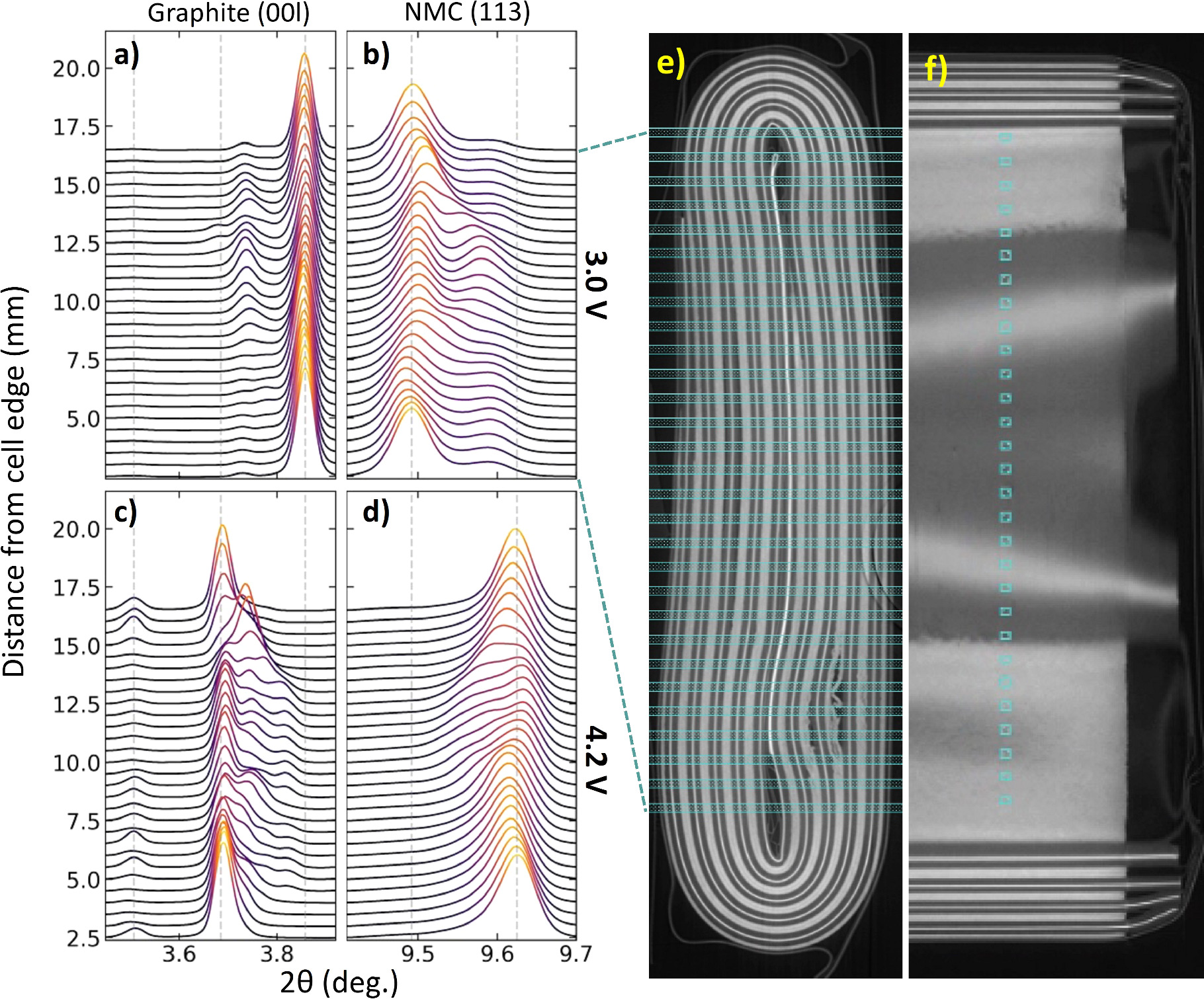
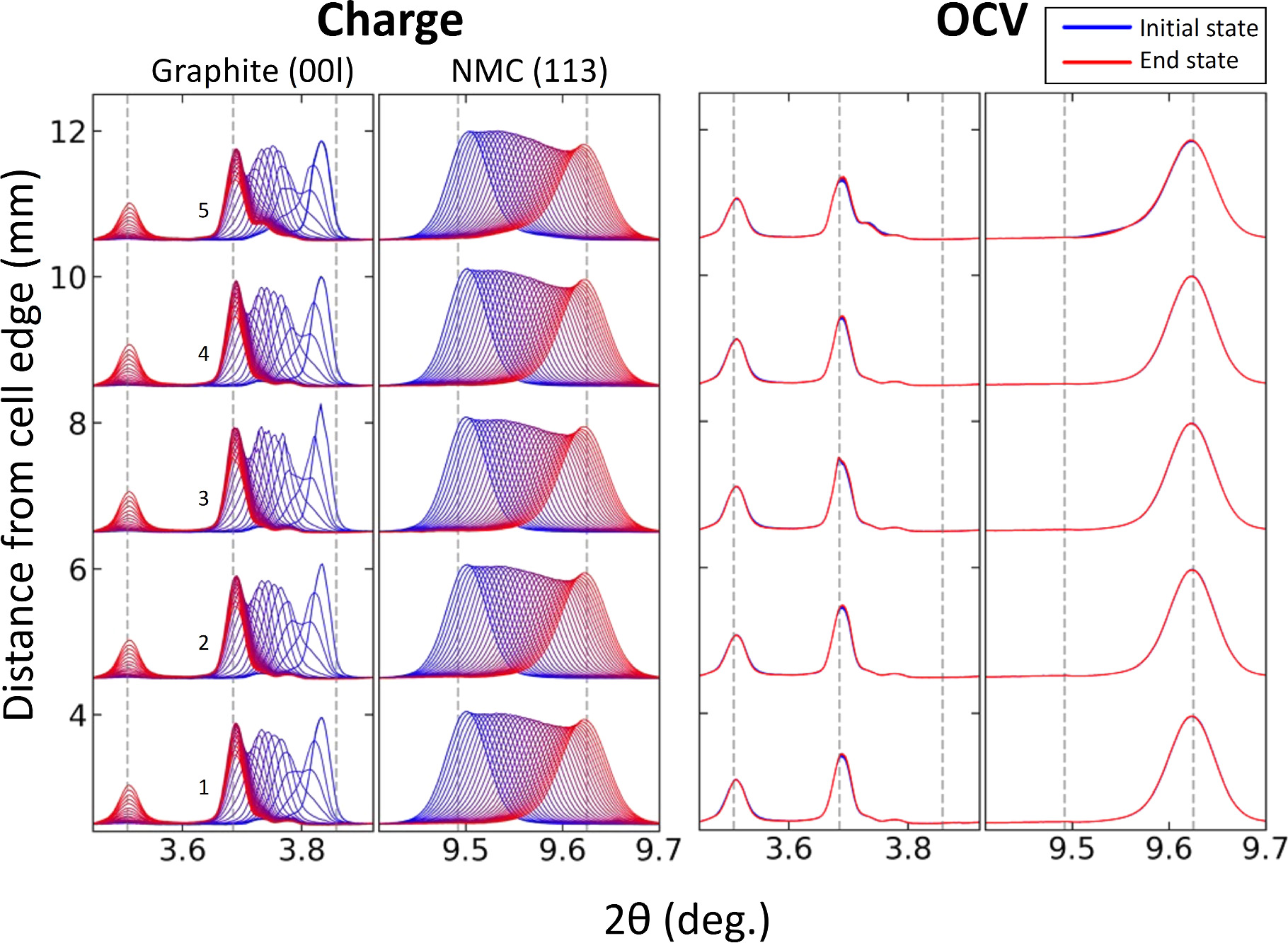
Figure 24. Comparison of operando XRD mapping data for (a) the single-crystal NMC532 cell that was cycled over 20,000 times vs (b) the "heavily cycled" polycrystalline NMC622 cell that was cycled 2380 times. These plots show evolution of the NMC (113) peak during CC-CV charge at C/3 from 3.0 V to 4.2 V (with a CV cut-off current of C/20). Each individual plot shows data that was collected at the indicated distance from the edge of the cell.
Download figure:
Standard image High-resolution image
Although signs of degradation and suppressed kinetics are visible in this cell, it is remarkable how minimal they are, given that it has undergone almost ten times the number of cycles as the polycrystalline NMC622 cell. Although both cells have lost ∼25% of their original capacity, the lithiation kinetics of the polycrystalline cell are complex and highly variable, while those of the single-crystal cell are simple, consistent, and spatially uniform. This result further reinforces the correlation between microcracking and the observed spatially heterogeneous kinetics.
Results like this are highly relevant for applications like second-life ESS facilities, where used cells and packs are repurposed for grid-storage applications. If, for example, the operator of a second-life ESS was to assess the suitability of these two cells by simply measuring their capacity, they would appear to have degraded by the same amount. But the above data indicates that the polycrystalline cell would be at a much higher risk for rollover failure, due to the larger exposed cathode surface area and a larger cathode pore volume that exceeds the volume of electrolyte in the cell. That cell would also likely be much more difficult for a battery management system (BMS) to model, due to the highly complex variations in lithiation kinetics. The single-crystal cell would be a much better candidate for second-life applications, as it would likely continue to operate and degrade in a predictable fashion that should be easily managed by a BMS. Thermal management of the polycrystalline cell could also be challenging if the observed heterogeneous kinetics lead to thermal gradients across the cell. The use of single-crystal materials in this case has not only improved the cycle life of the cell by an order of magnitude—it has produced an "end-of-life" cell that is much more suitable for use in a second-life ESS.
Conclusions
An overarching theme of this work is that heavily cycled commercial cells can show remarkable spatial heterogeneity and complex kinetic behavior, even within a single cell. Lab-based XRD measurements of such cells will be spatially averaged, while single-point synchrotron measurements will only sample a small portion of the cell and could lead to non-representative or even misleading results. To properly characterize degradation this extensive in commercial cells, spatially resolved experiments are needed to fully capture and isolate different behaviors in different regions of the cell. The combination of both spatially and temporally resolved experiments is a powerful tool for understanding non-equilibrium behavior. This is an application to which synchrotron XRD is uniquely suited.
Modelling the complex, multi-faceted behavior of extensively degraded cells is challenging. Assumptions cannot be easily made about the number of components present, their kinetic behavior, or their spatial distribution in the cell. Models that require such assumptions can work well for cells that have been cycled less extensively or under less abusive conditions, but heavily degraded cells like the one studied here do not easily lend themselves to this approach. Conducting a variety of both near-equilibrium and non-equilibrium experiments provides complementary information that is useful for validating assumptions and constructing appropriate models.
In this study, we included representative data on a heavily cycled cell with a single-crystal positive electrode to illustrate that the inactive fractions of the positive electrode can be extremely small, even after 20,000 cycles. Readers must realize that the choice of electrode materials and electrode formulations plays a dominant role in determining possible active mass loss during extended charge-discharge cycling.
Despite the complexity and challenge of characterizing such cells, this type of work will become increasingly relevant as more EVs reach end of life, and the supply of potential second-life battery packs grows over time. This work is meant to provide an appreciation for the complex behavior of heavily degraded cells, which require a cautious and nuanced approach to characterization and modelling. We hope the experimental protocols, data reduction techniques, and modelling approaches discussed here will be of use to other researchers trying to characterize the emergent properties of extensively degraded cells. As cycle-intensive applications like second-life ESS and V2G storage are implemented, a comprehensive understanding of these cells is becoming increasingly important.
Acknowledgments
The authors acknowledge the financial support of NSERC and Tesla Canada under the Alliance grant program. XRD and CT imaging work was carried out at the Canadian Light Source, which is supported by the Canada Foundation for Innovation (CFI), NSERC, the National Research Council (NRC), the Canadian Institutes of Health Research (CIHR), the Government of Saskatchewan, and the University of Saskatchewan. The authors would like to thank Al Rahemtulla and Sergey Gasilov of the CLS for their contributions to this work.